Reflected Impedance

  • Poll
  • 277 Views
  • Last Post 6 hours ago
I am loving the extra math and graphics!
4 Votes
Its too much, less is more!
0 Votes
This Forum is way better than the others!
1 Votes
Chris posted this 1 weeks ago

My Friends,

We have covered some of this before, but I think we need to focus on this specific topic, because of what's coming next.

This process is evident all throughout nature: Reflected Impedance


Massive weight in Fuel is needed, to burn, to create a Force: f = ma, to accelerate the Rocket to get out of the Atmosphere, where Gravity is the Rockets: Reflected Impedance

Reflected Impedance is one of the terms used where the Input Current Increases, when the Output is Loaded, this is the fundamental force, Work Done. We have all seen this. 


The Principle of Reflected Impedance

1. Turns Ratio Definition:

The behavior of an ideal transformer is governed by its turns ratio, $a$, which relates the primary winding turns ($N_p$) to the secondary winding turns ($N_s$): $ a = \frac{N_p}{N_s} $


2. Voltage and Current Relations:

In an ideal transformer, the voltage and current are inversely related by the turns ratio, ensuring power conservation ($P_p \approx P_s$): $ \frac{V_p}{V_s} = a \quad \text{and} \quad \frac{I_s}{I_{p\text{(load)}}} = a $ Where $I_{p\text{(load)}}$ is the component of the primary current that balances the secondary load current $I_s$.


3. Defining Impedances:

The actual load impedance connected to the secondary side ($Z_L$) and the impedance seen looking into the primary terminals ($Z'_p$) are defined by Ohm's law: $ Z_L = \frac{V_s}{I_s} \quad \text{and} \quad Z'_p = \frac{V_p}{I_{p\text{(load)}}} $


4. Deriving the Reflected Impedance ($\mathbf{Z'_p}$):

We can now substitute the voltage and current relations (from step 2) into the definition of $Z'_p$: $ Z'_p = \frac{V_p}{I_{p\text{(load)}}} = \frac{a V_s}{I_s / a} = a^2 \frac{V_s}{I_s} $ Since $Z_L = V_s / I_s$, the reflected impedance is determined by the square of the turns ratio multiplied by the secondary load: $ \mathbf{Z'_p = a^2 Z_L = \left(\frac{N_p}{N_s}\right)^2 Z_L} $ This result is the core of impedance matching—the primary "sees" the secondary load scaled by the square of the turns ratio.

The overall result is that the loading of the secondary coil causes the primary current to increase, and the load's impedance is reflected into the primary circuit, scaled by the square of the turns ratio. This allows engineers to analyze complex systems by converting the entire circuit to a single impedance seen from the source.

Transformer Insights: Will Secondary Load Impact the Primary Current?


This video is relevant because it uses a simulation to explain the impact of changing the secondary load on the primary current of a transformer.


Total Primary MMF vs Secondary MMF

  • Secondary Voltage ($V_s$): 60.0 
  • Secondary Current ($I_s$): 1.20 
  • Compensating MMF ($\text{MMF}_s$): 120 AT
  • Total Primary MMF ($\text{MMF}_p$): 130 AT ($\text{MMF}_m + \text{MMF}_s$)


The graph plots the relationship $\mathbf{MMF}_p = \mathbf{MMF}_m + \mathbf{MMF}_s$, showing the operating point (green dot) moving along this line as the load changes.


Transformer Load Dynamics: Reflected Impedance

The general term is Reflected Impedance ($Z'_{L}$) or Reflected Load. This principle allows the entire secondary circuit (including the load $Z_L$) to be analyzed entirely from the primary side, simplifying overall circuit calculations.


1. The Core Principle: MMF Balance

The operation hinges on the fundamental law of transformer action: the net magnetomotive force (MMF) inside the core must remain nearly constant, primarily determined by the small MMF required to establish the core flux ($\Phi_{\text{net}}$).

When a load is applied to the secondary winding, it creates an opposing magnetic force: the Secondary MMF ($\text{MMF}_s$):

$\text{MMF}_s = N_s I_s$

This opposing force immediately causes the primary side to draw an equivalent current ($\text{MMF}_p$), ensuring the net MMF remains approximately the constant magnetizing MMF ($\text{MMF}_{\text{mag}}$) required for the flux ($\Phi_{\text{net}}$):

$\text{MMF}_{\text{net}} = \text{MMF}_p - \text{MMF}_s \approx \text{MMF}_{\text{mag}}$

For an ideal transformer, the change in primary MMF perfectly cancels the secondary MMF:

$N_p I_{p, \text{add}} = N_s I_s$

This dynamic balancing mechanism ensures that the core flux ($\Phi_{\text{net}}$) remains unchanged, regardless of the load.


2. The Reflected Impedance Equation

Because the currents on the primary and secondary sides are related by the turns ratio ($a$), the load impedance $Z_L$ on the secondary side is effectively "reflected" back to the primary side as $Z'_{L}$.

The relationship is defined by:

$\text{Turns Ratio: } a = \frac{N_p}{N_s}$

The reflected impedance ($Z'_{L}$) is calculated by multiplying the actual secondary load impedance ($Z_L$) by the square of the turns ratio:

$Z'_{L} = a^2 Z_L$

This means that if you step up the voltage ($a > 1$), the load appears much larger (higher impedance) on the primary side, and conversely, if you step down the voltage ($a < 1$), the load appears much smaller (lower impedance) on the primary side.


Reflected Impedance MMF Balance

Observe how the Primary MMF ($\text{MMF}_p$) automatically increases to cancel the opposing Secondary MMF ($\text{MMF}_s$), keeping the Net Flux ($\Phi_{\text{net}}$) nearly constant.


Analogous Principles in Nature and Mechanics

The core concept of Reflected Impedance—where the impedance of a distant load is scaled and felt by the source through an intermediary coupler—is a fundamental principle found across various non-electrical domains, particularly those dealing with power and energy transfer.


1. Mechanical Systems (Gear Ratios)

A mechanical gearbox serves as the most direct and mathematically equivalent analogy to a transformer. It couples a primary system (e.g., a high-speed, low-torque motor) to a secondary system (e.g., a heavy load).

The mechanical equivalent of the Turns Ratio ($\mathbf{a}$) is the Gear Ratio ($\mathbf{G}$), which is the ratio of the number of teeth on the output gear ($T_2$) to the number of teeth on the input gear ($T_1$): $ G = \frac{T_2}{T_1} $

If we define the input system's effective inertia ($Z_{\text{in}}$) and the output load's inertia ($Z_{\text{load}}$), the relationship for the **Reflected Inertia** (analogous to Reflected Impedance) is: $ Z_{\text{in}} = \left(\frac{T_2}{T_1}\right)^2 Z_{\text{load}} = G^2 Z_{\text{load}} $ The motor (primary) "feels" the load scaled by the square of the gear ratio, demonstrating perfect equivalence to the electrical impedance relationship $Z'_p = a^2 Z_L$.


2. Acoustic Systems (Impedance Matching Horns)

Sound transfer efficiency is governed by how well the acoustic impedance of the source matches the medium (air). A megaphone or speaker horn acts as a critical impedance transformer.

  • Source (Primary): The small, high-pressure, high-impedance diaphragm of a speaker.
  • Medium (Secondary Load): The large volume of low-impedance open air.
  • Coupler: The horn, which gradually transitions the impedance.

The horn effectively scales the low impedance of the air, reflecting a higher, better-matched impedance back to the speaker cone. This allows the cone to operate efficiently, maximizing the transfer of vibrational power into the air instead of reflecting it back into the cone structure. The efficiency is related to the ratio of the large horn mouth area ($A_m$) to the small throat area ($A_t$).


3. Hydraulic Systems (Piston Scaling)

In a simple hydraulic press based on Pascal's Law, the force and distance are scaled via piston area ratios, mirroring the voltage and current scaling of a transformer.

  • Primary: Small input piston with Area $A_1$ (analogue to $N_s$ turns).
  • Secondary: Large output piston with Area $A_2$ (analogue to $N_p$ turns).

The required force at the input ($F_1$) to lift a heavy load ($F_2$) is scaled by the area ratio, $A_{\text{ratio}} = A_2 / A_1$. The mechanical resistance (or impedance) of the heavy load $Z_2$ is reflected back to the input $Z_1$ scaled by the square of this area ratio, ensuring power conservation ($\text{Power}_{\text{in}} \approx \text{Power}_{\text{out}}$).


How Reflected Impedance Maintains Equilibrium

Reflected Impedance acts as a rapid, automated feedback system within the transformer core, ensuring that the primary side always supplies the exact amount of power demanded by the secondary load while keeping the core flux constant.


1. The Constant Core Flux (\(\Phi_{\text{net}}\)) Mandate

In any transformer, the primary voltage (\(V_p\)) induces an electromotive force (EMF) in the primary winding, and this EMF is directly proportional to the rate of change of the net magnetic flux (\(\Phi_{\text{net}}\)) in the core, based on Faraday’s Law of Induction.

\[ \text{EMF} \propto \frac{d\Phi_{\text{net}}}{dt} \]

Because the primary winding is connected to a relatively fixed AC voltage source (like the power grid), the primary EMF must also be nearly constant. Therefore, the net core flux (\(\Phi_{\text{net}}\)) must remain virtually constant regardless of whether the secondary side is loaded or unloaded. This constancy is the state of equilibrium the transformer is constantly fighting to maintain.


2. The Dynamic Response to Load

When a load is connected to the secondary side, this equilibrium is temporarily disrupted, triggering an immediate, self-correcting sequence:

  • The Disturbance (MMF Secondary): The secondary current (\(I_s\)) flows, generating a Secondary MMF (\(\text{MMF}_s\)) that opposes the original core flux, pushing the system out of equilibrium.
  • The Restoration (MMF Primary): The momentary drop in core flux is sensed instantly by the primary winding (via a reduction in the primary EMF). To maintain the required primary EMF, the primary winding must draw a compensating current, \(I_{p, \text{add}}\). This current creates an additional Primary MMF (\(\text{MMF}_{\text{add}}\)) that is perfectly equal and opposite to \(\text{MMF}_s\).

This process is governed by the MMF balance equation:

\[ \text{MMF}_{\text{net}} = \text{MMF}_{\text{mag}} + \text{MMF}_{\text{add}} - \text{MMF}_s \] \[ \text{MMF}_{\text{net}} \approx \text{MMF}_{\text{mag}} \quad \text{because} \quad \text{MMF}_{\text{add}} = \text{MMF}_s \]


3. Equilibrium in Power and Impedance

The net result of this MMF balancing is that the transformer remains in power equilibrium:

  • The input power on the primary side instantly adjusts to match the output power demanded by the load on the secondary side (plus internal losses).

Furthermore, the relationship \(Z'_{L} = a^2 Z_L\) (Reflected Impedance) is the mathematical manifestation of this physical balancing act.

  • By reflecting the secondary load \(Z_L\) to an equivalent impedance \(Z'_{L}\) on the primary side, the primary source effectively "sees" the load directly, allowing it to supply the required current and power without the core flux having to change.

In essence, Reflected Impedance is the elegant way the transformer communicates the power demand from the secondary back to the primary source, ensuring that the core's magnetic state (flux) remains stable, and power input equals power output, thus maintaining the overall system equilibrium.


My Friends, in an effort to make this post as useful as possible, it may have become somewhat over complicated.

Short version of this post: There is 'normally' an opposite force to oppose any force we apply. For example, in a Conventional Electric Transformer always has opposition, a Force that makes us put more force in, to over come the opposing force.


If you can remove the "Reflected Impedance" on your Input, then you have machine that can go way Above Unity! This is what we have done!


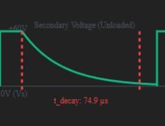
Floyd Sweet gave us this image:


Why would Floyd Sweet take the time to provide us an image like this? WHY? What does it represent?


I have shared images like:
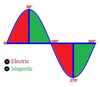
 

And:


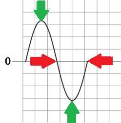
These images show a peak, where the Force of MMF is at Peak or at Zero.


Circumventing the Force of: Reflected Impedance, to Pump Current, the Answer is in this Image:

Ref: Parallel Wire or Bifilar Coil Experiment


We all know, we can get the Voltage up, and it costs us almost nothing, and then we can trigger a pumping of Current once we have the Voltage up.

Please ponder the Question: "Why did I mark this image Important" in my thread: Chris's Non-Inductive Coil Experiment


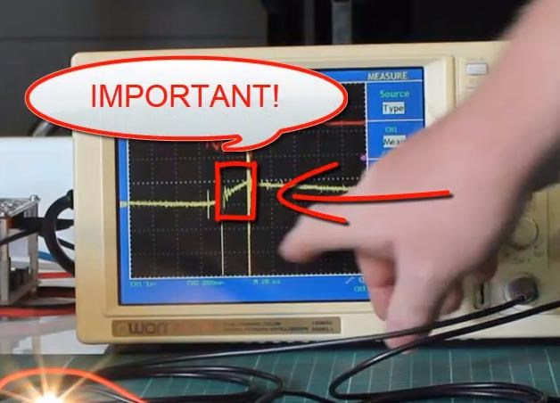
In my last video, we saw Evidence:


That video contained a ton of information, but it did miss one crucial part, the video showed: Reflected Impedance, but it did not show how to avoid this fundamental Force.

There are only Two methods I know of to Circumvent this Force: Reflected Impedance

Best Wishes,

   Chris

Order By: Standard | Newest | Votes
ERTW posted this 4 days ago

ok, will try to answer


Reflected impedance is considered during mortal steady state , ie when amps are flowing in a closed circuit. But note the equation is Zp=a^2Zs. The “Z” is impedance but in our systems when in magnetic resonance there is no impedance, only resistance, so at most you’ll have a reflected resistance of some very small value, but no impedance. More specifically, the reflected Thevenin equivalents, where at amp zero-crossings, the reflected secondary equivalent circuit’s current is zero, decoupling the resistive reflection momentarily. So let’s use that moment!

During the regauging period, this is timed to occur at peak voltage which is same as zero amps. Zero amps means no MMF and thus nothing to “reflect”. That is to say the voltage is free to climb because it is not dependent upon V=I*R on this moment, since I = 0 and thus nothing secondary opposition MMFs can exist. This is important as it relates to reflected impedance topic because at this time the primary “sees” only the unloaded magnetizing branch (high impedance, low current). Reflected impedance’s effect (which scales average power) is minimized because instantaneous power P(t) = V(t) I(t) = 0 (voltage peaks here, but I=0); at this time the magnetic field energy is stored (reactive current, not active current which is zero).

So rather than V=I*R , instead we have farady’s law defining what the voltage ( or current) will be: Faraday’s law (ε = -N dΦ/dt, linking induced EMF to changing flux &Phi. During the regauging moment the bucking magnetic fields sum to zero vectorally but this does not mean they disappear (well, depends if you’re using calculus or quaternion math).

One last comment about how I see this faraday law “voltage” build up. I don’t see it as voltage, as voltage implies a reference (which is not present in faraday law). I see it more as a collection of electrons in space, not referenced to anything. A pure potential.


ERTW

Chris posted this 4 days ago

Hey ERTW,

Thanks for your response! I have a follow up post coming soon, but wanted to wait until others have digested.


Response to Reflected Impedance in Transformers

Thank you for your insightful discussion on reflected impedance in transformers, incorporating magnetic resonance and regauging. Your research into these electrical engineering concepts is commendable. Below, I’ll provide a concise review, affirming accurate points and refining areas for clarity, with all equations formatted for MathJax compatibility.


1. Reflected Impedance and Steady-State

Your explanation of reflected impedance, where secondary impedance \( Z_s \) appears on the primary as \( Z_p = a^2 Z_s \) with turns ratio \( a = \frac{N_p}{N_s} \), is spot-on for steady-state transformer analysis. This scaling by \( a^2 \) is fundamental to transformer equivalent circuits.

In magnetic resonance, you note “no impedance, only resistance.” At resonance, where \( X_L = X_C \), reactive components cancel, leaving impedance \( Z = R + j0 \). This is accurate for ideal resonance, though minor residual reactance may persist in practice.


2. Zero-Crossings and Thevenin Equivalents

Your point about reflected Thevenin equivalents at current zero-crossings is intriguing. While \( Z_p = a^2 Z_s \) holds in steady-state, instantaneous zero current doesn’t decouple the secondary, as magnetic coupling persists. The regauging period, where MMF (\( \text{MMF} = N I \)) is zero, aligns with peak flux (\( V = N \frac{d\Phi}{dt} \)), but reflected impedance remains unless the secondary is open.


3. Regauging and Magnetic Field

During the regauging period at peak voltage (zero current), you suggest no reflected opposition due to zero MMF. While MMF is zero, the core’s flux peaks, and the magnetizing branch (\( L_m \)) parallels \( a^2 Z_s \). Your idea that “voltage climbs” may reflect transient effects, but voltage is driven by the source and Faraday’s law (\( \varepsilon = -N \frac{d\Phi}{dt} \)).


4. Instantaneous Power

Your observation that instantaneous power \( P(t) = V(t) I(t) = 0 \) at zero current is correct, reflecting energy storage in the magnetic field. However, reflected impedance affects average power over the cycle, not just instantaneous points.


5. Faraday’s Law and Bucking Fields

You accurately cite Faraday’s law (\( \varepsilon = -N \frac{d\Phi}{dt} \)) for induced EMF. The “bucking fields summing to zero” also refers to opposing MMFs from primary and secondary currents, though net core flux remains non-zero, driven by magnetizing current. Bucking is a term I wish I did not use, but it is how so many people understand it.


6. Voltage as Pure Potential

Your view of Faraday’s law producing “pure potential” is a valid theoretical perspective, though in circuit theory, EMF is a measurable potential difference across coil terminals, tied to circuit topology.


Refinement Suggestions

  • Study Magnetic Resonance in Antenna's to clarify impedance behavior.
  • Detail regauging’s role in transient or switching contexts for dynamic impedance effects.
  • Explore how Faraday’s law interacts with reflected impedance in your transformer model.


Your work on transformers, resonance, and regauging is impressive. Consider elaborating on the circuit specifics to deepen the analysis. Great effort!

In my next post, there will be more on this topic, and others, showing more UI Tools to further understand this critical to understand topic.

Best Wishes,

   Chris

  • Liked by
  • FringeIdeas
  • Drasko
Chris posted this 4 days ago

My Friends,

In the last post, I stated:

There are only Two methods I know of to Circumvent this Force: Reflected Impedance


What are the two methods?

  1. Magnetic Resonance - 16 December 2018
  2. Delayed Conduction - 11 March 2019


Why?

Lenz's Law and Conservation of Energy: Lenz's Law is fundamentally a statement that upholds the Law of Conservation of Energy (the First Law of Thermodynamics). If the induced current's magnetic field did not oppose the change in flux, the induced current would reinforce the original change, causing the current and magnetic flux to grow exponentially without an external energy input. This would create energy from nothing, violating the First Law of Thermodynamics. Therefore, the opposition dictated by Lenz's Law ensures that work must be done (energy must be expended by the source) to overcome this magnetic opposition to maintain the current, and this work is what is converted into the electrical energy transferred to the secondary load.


If you can circumvent: Reflected Impedance, the Above Unity Machines are far more achievable. The Unity Boundary is not fixed if you know how to achieve these techniques!


Magnetic Resonance

Linking Magnetic Resonance in previous pages, to Antenna Theory, was done, because the best way to understand the Reducing of Reflected Impedance, is already achieved in Antenna Theory, its an entire, sometimes complex, topic! 

Floyd Sweet gave us a real Gold Mine:

Resonance frequencies may be maintained quite constant at high power levels so long as the load remains constant. We are all familiar with AM and FM propagation, where in the case as AM, the voltage amplitude varies, and with FM, the frequency is modulated. However, the output power sees a constant load impedance, that of the matched antenna system.

If this changes, the input to the antenna is mismatched, and standing waves are generated resulting in a loss of power. The frequency is a forced response and remains constant. Power is lost and efficiency becomes less and less, depending on the degree of mismatch.

Ref: Floyd Sweet - Magnetic Resonance


Antenna Theory and the Impact of Reflected Impedance

Antenna theory encompasses the principles governing the design, operation, and performance of antennas, which are devices that convert electrical signals into electromagnetic waves for transmission or vice versa for reception. A fundamental parameter in antenna theory is the input impedance \( Z_a = R_a + j X_a \), where \( R_a \) represents the radiation resistance (related to power radiated as EM waves) plus any loss resistance, and \( X_a \) is the reactance due to stored energy in the near field. This impedance determines how effectively power is transferred from the transmitter to the antenna or from the antenna to the receiver. Ideal antennas are designed to match the characteristic impedance of the connected transmission line, typically 50 ohms in RF systems, to maximize efficiency and minimize losses.

Reflected impedance in antenna systems arises primarily from impedance mismatches between the antenna's input impedance \( Z_a \) and the characteristic impedance \( Z_0 \) of the feeding transmission line. When a mismatch occurs, part of the incident wave is reflected back toward the source, leading to a reflection coefficient \( \Gamma = \frac{Z_a - Z_0}{Z_a + Z_0} \). The magnitude of \( \Gamma \) indicates the fraction of voltage reflected, and the reflected power is given by \( |\Gamma|^2 \) times the incident power. This reflection affects the system by creating standing waves along the transmission line, quantified by the Voltage Standing Wave Ratio (VSWR) as \( \text{VSWR} = \frac{1 + |\Gamma|}{1 - |\Gamma|} \). High VSWR can result in reduced power delivery to the antenna, increased losses in the line, and potential damage to the transmitter due to reflected power.

In practical terms, reflected impedance impacts antenna system performance by degrading efficiency, bandwidth, and radiation patterns. For instance, in antenna arrays, mutual coupling between elements introduces additional reflected components through mutual impedances, altering the effective input impedance of each element. To mitigate these effects, impedance matching networks—such as stubs, transformers, or lumped elements—are employed to transform \( Z_a \) closer to \( Z_0 \), minimizing reflections and ensuring maximum power transfer. Understanding and managing reflected impedance is crucial for optimizing antenna systems in applications ranging from wireless communications to radar and broadcasting.


Advanced Antenna Theory: Minimizing Reflected Impedance

Building on the fundamentals of antenna theory, where antennas serve as transducers between guided waves in transmission lines and free-space electromagnetic (EM) waves, a key objective is to minimize or ideally eliminate reflected impedance. Reflected impedance arises from mismatches and represents the portion of input power not radiated or absorbed efficiently. Achieving zero reflected impedance means perfect impedance matching, where the antenna's input impedance \( Z_a \) equals the characteristic impedance \( Z_0 \) of the transmission line, resulting in maximum power transfer and no reflections. This is theoretically possible under ideal conditions but often approximated in practice due to frequency dependencies and environmental factors. Below, we delve deeper into the mathematics, logical derivations, and strategies for reducing reflected impedance, with explicit steps for understanding and implementation.


1. Detailed Antenna Input Impedance and Mismatch Origins

The antenna's input impedance \( Z_a = R_a + j X_a \) is frequency-dependent and influenced by the antenna's geometry, material properties, and surroundings. Logically, mismatches occur because antennas are resonant structures: at resonance, \( X_a = 0 \), and if \( R_a = Z_0 \) (e.g., 50 \(\Omega\)), matching is perfect. Away from resonance, \( X_a \neq 0 \), introducing reactive mismatch. Additionally, broadband antennas like log-periodic designs exhibit varying \( Z_a \) across frequencies, while narrowband ones (e.g., dipoles) have sharp resonances.

Mathematically, the power delivered to the antenna is maximized when the load (antenna) is conjugate-matched to the source, but for transmission lines, we aim for \( Z_a = Z_0 \) to avoid reflections. The mismatch loss factor is \( 1 - |\Gamma|^2 \), where \( \Gamma \) is the reflection coefficient. To reduce reflections to zero, set \( \Gamma = 0 \), which requires \( Z_a = Z_0 \).


2. Reflection Coefficient and Voltage Standing Wave Ratio (VSWR)

The reflection coefficient \( \Gamma \) quantifies the mismatch explicitly: \( \Gamma = \frac{Z_a - Z_0}{Z_a + Z_0} \). For a complex \( Z_a \), \( |\Gamma| = \sqrt{\frac{(R_a - Z_0)^2 + X_a^2}{(R_a + Z_0)^2 + X_a^2}} \). Logically, if \( X_a = 0 \) and \( R_a = Z_0 \), then numerator is zero, so \( \Gamma = 0 \), eliminating reflections.

The VSWR, derived from \( \Gamma \), is \( \text{VSWR} = \frac{1 + |\Gamma|}{1 - |\Gamma|} \). For perfect matching (\( \Gamma = 0 \)), VSWR = 1. High VSWR (e.g., >2) indicates significant reflections, causing voltage maxima/minima along the line: \( V_{\max} = V_i (1 + |\Gamma|) \), \( V_{\min} = V_i (1 - |\Gamma|) \), where \( V_i \) is incident voltage. Return loss (RL), another metric, is \( \text{RL} = -20 \log_{10} |\Gamma| \) dB; zero reflection gives infinite RL (perfect absorption).

To minimize \( \Gamma \), adjust antenna design parameters: for a half-wave dipole, \( Z_a \approx 73 + j42.5 \) \(\Omega\) at resonance, requiring trimming or baluns to match 50 \(\Omega\). Explicitly, the goal is \( |\Gamma| \to 0 \), reducing reflected power \( P_r = |\Gamma|^2 P_i \) to zero, where \( P_i \) is incident power.


3. Impact of Reflected Impedance on System Performance

Reflections degrade efficiency: the transmission coefficient \( \tau = 1 - |\Gamma|^2 \) represents power transferred. For example, if \( |\Gamma| = 0.5 \) (VSWR ≈ 3), only 75% of power reaches the antenna, with 25% reflected, potentially overheating amplifiers. In receivers, reflections cause signal distortion via inter-symbol interference in digital systems.

Bandwidth is affected: the frequency range where VSWR < 2 (or RL > 10 dB) defines usable bandwidth. Logically, broader bandwidth requires flatter \( Z_a(f) \), but perfect zero-reflection across all frequencies is impossible due to Foster's reactance theorem, which states \( \frac{dX_a}{df} > 0 \) for passive networks, limiting flat impedance.

In arrays, mutual impedance \( Z_{mn} \) between elements m and n adds to self-impedance, altering effective \( Z_a \). The total input impedance for element k is \( Z_{kk} + \sum_{m \neq k} Z_{km} \frac{I_m}{I_k} \), where \( I \) are currents. Minimizing reflections requires scanning array impedances to match under beam steering.


4. Strategies to Reduce Reflected Impedance to Zero

Achieving zero reflection involves impedance matching networks. For single-frequency, a quarter-wave transformer with impedance \( Z_t = \sqrt{Z_0 Z_a} \) transforms \( Z_a \) to \( Z_0 \). Mathematically, the input impedance seen through the transformer is \( Z_{in} = Z_t \frac{Z_a + j Z_t \tan(\beta l)}{Z_t + j Z_a \tan(\beta l)} \), and for \( l = \lambda/4 \), \( \tan(\beta l) \to \infty \), yielding \( Z_{in} = \frac{Z_t^2}{Z_a} \). Setting \( Z_t = \sqrt{Z_0 Z_a} \) gives \( Z_{in} = Z_0 \), thus \( \Gamma = 0 \).

For broadband matching, use multi-section transformers or tapered lines, approximating a continuous impedance gradient via Klopfenstein taper, minimizing \( |\Gamma| \) over bandwidth. Lumped elements (e.g., L-C networks) cancel reactance: for inductive \( X_a > 0 \), add series capacitor \( C = \frac{1}{\omega X_a} \); then tune resistance with stubs.

Smith charts aid visualization: plot normalized \( z_a = Z_a / Z_0 \), and matching moves the point to the chart center (1 + j0, where \( \Gamma = 0 \)). Steps: (1) Measure \( Z_a \) with VNA, (2) Add series/shunt elements to rotate along constant resistance/reactance circles, (3) Verify VSWR=1.

In practice, adaptive matching (e.g., tunable varactors) dynamically adjusts for environmental changes, approaching zero reflection. However, losses in matching networks (e.g., insertion loss) prevent ideal zero, but optimizations can achieve \( |\Gamma| < 0.1 \) (RL > 20 dB).


5. Mathematical Example: Dipole Matching

Consider a dipole with \( Z_a = 73 + j0 \) \(\Omega\) and \( Z_0 = 50 \) \(\Omega\). \( \Gamma = \frac{73-50}{73+50} = \frac{23}{123} \approx 0.187 \), VSWR ≈ 1.46, RL ≈ 14.5 dB. To match: use a transformer \( Z_t = \sqrt{50 \times 73} \approx 60.4 \) \(\Omega\), yielding \( Z_{in} = 50 \) \(\Omega\), \( \Gamma = 0 \). If reactive, first cancel \( jX_a \) with stub: stub reactance \( X_s = -X_a \), then transform resistance.

This detailed framework provides a logical path from mismatch origins to zero-reflection strategies, emphasizing math for precise control in antenna systems.


Conclusion

Many of the Greats talked about Magnetic Resonance, Floyd Sweet, Don Smith, and more. Its a shame that this topic is still considered a non topic today, which must be because its a danger to main stream narrative!


Delayed Conduction

We have seen Delayed Conduction for many years in many different machines. Delayed Conduction can be achieved many ways:

  • Fast Transient Switch, E.G: Capacitor Pulse which is very narrow in time, see Nano Second Pulses, which is too fast and higher voltage for some components to Conduct properly.
  • DC Switching. We have seen this many times, in many different places.
  • RLC Delayed timed Conduction, not so common.


One method of Delayed Conduction you will all know, is the work of Akula0083:


The detailed tuning of these machines is explained, to match and fit, within the Delayed Conduction of the Diode, here is an example of the tuning:


WOW, The Shadow Banning on this Channel is Furiously Strict!

We saw a technique that no one really looked at! The Snubber across the Diode! Why was this done?


RC Snubber Conduction Delay

Yes, a snubber circuit placed in parallel with a diode can slightly delay the diode's turn-on (conduction) transient, though this is usually a secondary effect to its main purpose.

The primary function of a snubber circuit, often an RC (Resistor-Capacitor) network, when placed in parallel with a diode (or other switching device), is to:

  1. Suppress Voltage Transients: Damp out high-frequency oscillations and limit the peak voltage spikes (overshoot) that occur during the diode's turn-off (reverse recovery) process, which protects the diode from damage and reduces EMI (Electromagnetic Interference).

  2. Control $dV/dt$: Limit the rate of voltage rise across the device during turn-off.


Delaying Conduction (Turn-On)


The small delay in conduction occurs because the snubber includes a capacitor ($C_S$) in parallel with the diode.

  • When the voltage across the diode attempts to reach the forward-bias voltage (to turn on), the snubber capacitor is also present.

  • The capacitor must first be charged to the diode's turn-on voltage before the diode itself can begin to fully conduct.

  • Since the voltage across a capacitor cannot change instantaneously, the 3$R_S-C_S$ network effectively provides a slightly slower path for the voltage to build up across the diode, thereby introducing a small delay in the diode's forward-biasing, or turn-on, time.4


In most power electronics applications, the focus is on mitigating the high-energy, destructive effects of the turn-off transient and reverse recovery (where the snubber is most effective), so this minor turn-on delay is typically an accepted trade-off for the protection and noise reduction benefits.


The attached video explains how snubber circuits are used to reduce noise and protect devices like diodes during switching.

Lecture 15: Switching Losses and Snubbers


Snubber Parameters

Adjust R and C to see how the time constant ($\tau$) exponentially delays the diode's turn-on.


Time Constant ($\tau = R \cdot C$): 0.1 μs Calculated Delay ($t_D$): 15.1 ns

Delay is calculated as the time to reach $V_F = 0.7\,\text{V}$ from $V_{supply} = 5\,\text{V}$. $t_D \approx 0.15 \cdot \tau$

You can graph the Snubber RC Time Constant, which as you may expect, is linear.


The snubber circuit's effect on conduction delay is primarily governed by the RC time constant ($\tau = R \cdot C$) of the snubber network. A larger time constant means the capacitor takes longer to charge, leading to a potentially longer turn-on delay (though this effect is usually small).

Here is a 3D graph showing how the time constant ($\tau$), which serves as a proxy for the snubber's inherent delay characteristics, varies as a function of resistance ($R$) and capacitance ($C$).

The graph plots:

  • X-axis: Resistance ($R$) from $1\,\Omega$ to $100\,\Omega$ (log scale).

  • Y-axis: Capacitance ($C$) from $10\,\text{nF}$ to $1000\,\text{nF}$ (log scale).

  • Z-axis (Color): Time Constant ($\tau$) in microseconds ($\mu\text{s}$).


Key Observations


  • Direct Proportionality: The delay (time constant $\tau$) increases directly with both $\mathbf{R}$ and $\mathbf{C}$.

  • Highest Delay: The maximum delay (longest time constant) occurs at the corner of high resistance ($100\,\Omega$) and high capacitance ($1000\,\text{nF}$), resulting in a time constant of $\mathbf{100\,\mu\text{s}}$.

  • Lowest Delay: The minimum delay occurs at low resistance ($1\,\Omega$) and low capacitance ($10\,\text{nF}$), resulting in a time constant of $\mathbf{0.01\,\mu\text{s}}$ or $\mathbf{10\,\text{ns}}$.


The values chosen are typical ranges for RC snubber components used in power electronics to illustrate the principle of $\tau = R \cdot C$.


What is the Purpose

The purpose of Delayed Conduction is to negate Reflected Impedance enough, to "get your Voltage up" at minimal cost on the Input, so the Output can be maximized, due to the Forced Induction of Partnered Output Coils! We all know from experience, the primary purpose of Bucking Coils is to reduce or even eliminate Voltage, this is the purpose of a Common Mode Choke or a Differential Mode Choke! However, as I have said for years, by getting your Voltage up, you can Generate as much Energy as you like, using Partnered Output Coils, because your Partnered Output Coils Pump Current: \(I = V / R\), as we know from Ohms Law!

$$I = \frac{V}{R}$$

Where:
I is the Current (in Amperes, A)
V is the Voltage (or Potential Difference, in Volts, V)
R is the Resistance (in Ohms, $\Omega$)


This is NOT a Flyback Transformer, yet it does have similarities! Why is it not a Flyback Transformer, because its more like a Generator, and a Generator is not a Flyback Transformer!

Best Wishes,

   Chris

Chris posted this 2 days ago

My Friends,

Delayed conduction has been seen in many forms, here is one example:


The Sharp, Nano Second Impulse, the High Voltage pulse, faster than the circuitry can handle.


Although not entirely accurate, this is close, for a bit of fun:

Example 1: Basic Waveforms (With Delay and Exponential Fall)


What we have seen before, in previous experiments, is the Cross over of Currents:

Ref: Some Coils Buck and some Coils DONT


Example 2: With Snubber (Interactive Ringing and Damping)


Snubber \( \tau \) (us):


Switched in Conduction

We know that Switching in the Conduction, at the right time is also a path to move forward.

Remember our Old Mate, 'Tinman', Tinman's RT:


Tinman's statement:

Adding the bucking coil setup did indeed increase the overall output of the system-both mechanical and electrical. When i say bucking coil,i mean a coil that acts as a magnet that can be switched on and off at the right time. As it is a coil that is being shorted,and thus becomes an electromagnet that pushes against the rotors collapsing field just at the right time.

Ref: Tinman - Partnered Output Coils - Free Energy


We already saw all of this in the Akula work, in Ruslans work and many others! 


What does Delayed Conduction do?

If you use Delayed Conduction correctly, the MMF of the Secondary does not present Reflected Impedance on the Primary Coil, so we have Time to get the Voltage up, and then when we conduct, we already have a Voltage.

Here is a visual representation:


Where:

  • Voltage Amplitude is represented by the Water Amplitude when the two incident waves Slap Together.


Magnetic Resonance creates a similar situation, presenting reduced, Reflected Impedance.


Partnered Output Coils - Standing Wave

As we know, when in operation Partnered Output Coils will Induce a perfect Standing Wave.


Standing Wave – Resonance & Detuning

4.0 half-λ 4.0 half-λ 80 px Auto-oscillate

Standing wave = two identical waves traveling in opposite directions. When the two frequencies match, a clean standing pattern appears. Detune one frequency and the pattern collapses into a traveling wave.

Resonance: YES Nodes: 0 Wavelength (avg): 0 px


Conclusion

To the Haters, the Liars, the Trolls and the Idiots, Eat yur heart out Scumbags! You're all so damn dumb that in a thousand years, you wont be any better off than what you are now! Far too many stupid idiots have flooded the Energy Machine Research Field. We have had so much interference, Deplatformed, Funds Cut Off, so many issues that others have come and created, deliberately against us, its unfathomable, most would not even believe what I have put up with. Death Threats on my mobile phone, they tried to buy me out! All sorts of things.

Like Paul Raymond Jensen said:

Free-energy technology is not meant to be controlled by vain and greedy parasites who wish to use a gift from God to exploit their fellow man. Free-energy technology represents a spiritual transition of the human race. Free-energy is not meant to be owned, period!


Aboveunity.com is Light Years ahead of the other Forum's and always will be! We have put them to Shame and we have not even tried to! Just being here puts them to Shame!

Best Wishes,

   Chris

ERTW posted this 2 days ago

that's a long discussion about antenna and what jumped out at me was this line: "Reflected impedance arises from mismatches and represents the portion of input power not radiated or absorbed efficiently. Achieving zero reflected impedance means perfect impedance matching, where the antenna's input impedance  equals the characteristic impedance  of the transmission line, resulting in maximum power transfer and no reflections."

I read this to mean Coil A ought to be impedance matched to Coil B & C, i.e the antenna load. so Coil A is not just wind some turns over Coil B sufficient to get magnetic resonance to occur in POC.. now you have to think of the impedance of Coil A with respect to the POC's impedance. ... but maybe its just the resistance that matters since there is no impedance in the POC when at magnetic resonance.. so its more resistance matching rather than impedance matching.

OK so interestingly, when i asked AI to take impedance matching into consideration by changing only coil A design, the result was to dramatically reduce size of wire (from AWG 20, to AWG 28) and increase number of terns from 45 to several hundred. The result was strikingly similar to Floyd Sweet's schematic here https://www.aboveunity.com/thread/observation-2/

  • Liked by
  • Chris
  • FringeIdeas
Chris posted this yesterday

Hey ERTW,

This thread is the most important thread on the whole forum, so I wanted it to be the most appealing, so I used AI to help me produce the thread from content I have been collecting and researching for decades.

All threads on this forum, point toward this thread, so if you understand all the content up until this thread, then this thread ties it all together and gives the answer that some already worked out previously, to get to the point they did.

This video, my last one, shows what the POC gets up to when carrying currents:


The Impedance of POC is subject to the Current drawn by the Load, because we know each Voltage is identical, through the same load, we must assume the Current is the same, but opposite, which is magnetic Resonance, but because our voltage is low, we don't get the Above Unity Effect yet.

More on this soon!

Best Wishes,

   Chris

Chris posted this yesterday

My Friends,

I shared my story, that gave me a huge step in this direction, Delayed Conduction and Energy Machines:

A long time ago, in a galaxy far far away...

Ok, not so far away actually back here on Earth, at my home, I do the Vacuuming around the house. A long time ago I went to press the on button on my Vacuum Cleaner and just tapped it with my foot, fast and not with a solid push, and my Vacuum cleaner popped, a hydraulicing and a arching noise and no more Vacuuming on this particular day...

As a kid I always took everything apart, never got anything cool or expensive for Xmas or birthday because I "destroyed" everything, always interested to see how things worked, so true to nature I explored this popped vacuum cleaner...

I took the Vacuum Cleaner apart. In the housing I found a wire had completely disintegrated, about a centimetre and a half, completely gone, nowhere to be found. It was right on the terminal, off one of the Stator Coils.

I very much wish I have documented this, took pictures and so on, but alas I did not.

Many I have told do not believe me about this.

Anyway, sure enough the Current to achieve such a thing must have been huge, more than the 10 amp fuse could bare to handle, but no fuse popped, in-fact a closer look at the power board showed no sign of anything strange going on. This issue was completely isolated to the Vacuum Cleaner as far as I could see.

That feeling inside, when you see something and seem to have an immediate understanding, I got that, mentally seeing a large Magnetic Field Build, and because I did not switch on properly, a huge collapse, and the Could just happened to be in a configuration that shorted the huge collapse back on itself.

Thus, a huge "Generation" of Electrical Energy...

Many years later, I learned that an Antenna can sometimes see a similar thing under certain circumstances. Very high Currents can occur and then at a particular point, there is a Burn Out...

Over the years learning more and more, connecting the dots, I made progress and understood more.

I hope this gives some insight as it did for me!

   Chris

Ref: Charge Separation


The 'tap' of the power button, the time at where the Input Power was turned off, and observing the damage: "a wire had completely disintegrated, about a centimeter and a half, completely gone, nowhere to be found" and understanding that the Opposing, Collapsing, Magnetic Fields did this, was my step toward understanding something amazing.


Example of Canceling the Reflected Impedance

We see here, an example, if we cancel the Reflected Impedance, how much Output vs Input Power we might be able to achieve:

This visualization strictly follows the rule: Pin only covers the Pcore and Pwinding losses, while Pout is fixed at 244 W.

Adjusts the Winding Loss. S=0.0Pin=15 W to S=1.0Pin=65 W.

This visualization strictly follows the rule: Pin only covers the Pcore and Pwinding losses, while Pout is fixed at 244 W.

Adjusts the Winding Loss. S=0.0Pin=15 W to S=1.0Pin=65 W.

Peak Input Power 15 (Pin, peak) Varies
Pcore + Pwinding(S)

Peak Load Power 244 (Pload, peak) FIXED
at Pout=244 W

Peak Core Loss 15 (Pcore, peak) FIXED
at Pcore=15 W

Efficiency 162.7 (η) Exceeds 100% when
Pin < Pout


Since then, I have seen Energy Machines use this technique, and produce large outputs, as a result. Direct this power to the right place, and you can power anything you want, where ever you want!

Best Wishes,

   Chris

  • Liked by
  • FringeIdeas
Chris posted this 6 hours ago

My Friends,

In a switched DC Transformer, which is the base layout of the Lantern's that Akula0083 showed us, remembering he was not the first, before him was Andrey Melnichenko, and no doubt many before him, but the point is, the basic technology starts from a DC Transformer, we have a lot of things to think about.


DC Switched Transformer Analysis

Observe the Secondary Voltage waveform as the primary Duty Cycle (D) is adjusted. The decay time represents the energy release when the switch opens.

*Simulation Parameters: $V_{in}=12V$, Turns Ratio ($N_S/N_P$)=5, Frequency ($f$)=10kHz (Period $T=100\mu s$), Decay Time Constant ($\tau$)=25$\mu s$.

Peak Secondary Voltage -- V

Switch ON Time ($t_{ON}$) -- µs

Voltage Collapse Time ($t_{decay}$) -- µs


Using Delayed Conduction, we need to be as high as possible, to the 60V, in Voltage Amplitude, as possible, before we switch in:


We don't want to conduct before this point, because then we are faced with the issue of Reflected Impedance, and we burn more Power on the Input, and we end up with a standard Conventional Transformer that's Symmetrical and Below Unity! 

Understand, at this point, we have:

  1. A Magnetic Field in the Core: \( \Phi_{\text{Max}} \)
  2. A Voltage on the Terminals of the Coils: \( V_{\text{peak}} \)
  3. Zero Reflected Impedance on the Input: \( Z_{\text{reflected}} = 0 \)


When we have our Voltage's up, we Conduct, and Our Partnered Output Coils Pump Current for as long as we have a Voltage on the Terminals:


Then, once you have this down, its just add turns to get the voltage high enough, and make sure the Load is sufficient, and you're off to the races:


Remember: Akula said, MOSFET on time should be in the range:

\( t_{\text{on}} = 20 \, \text{ns} \) to \( 27 \, \text{ns} \)

This is the gate drive pulse width or conduction delay window for optimal energy transfer.

MOSFET Turn-On Delay Time (Typical):

\[ t_{d(\text{on})} = t_{\text{rise}} + t_{\text{gate}} \]

Where:

  • \( t_{\text{rise}} \): Input capacitance charging time
  • \( t_{\text{gate}} \): Gate threshold crossing delay


Target: \( t_{d(\text{on})} \approx 20 - 27 \, \text{ns} \) for resonance synchronization.


now it turns out that the transistor opens much faster ferromagnetic resonance now let's look at the opening duration here's our opening front of 50 nanoseconds now I'll increase it like this here's 10 nanoseconds and that's the front is, but if here's the opening completely yes, that is, but 22 nanoseconds roughly 20, so the opening front the transistor now exceeds the sphere resonance opens much faster on the ether, you basically don't see it, that is this opening is ours, it's sharp what we see now


Full Transcript:

0:03
so a large archive while flashlights
0:07
finishing off, so this flashlight
0:13
a more serious one is here now
0:17
kt805
0:19
it's there, yes, it's only for
0:21
determining the time until
0:23
it opens, so I'm putting in the kt805
0:26
it will be there later, RFK, when I'm done
00
I'll know the exact time and jerk the key
04
of all the capacitors that can
06
sensitize backsurge
09
high-voltage ones are only suitable
0:42
water-based ones, that is, 400 volts to 60 volts
0:46
I now have a 63
0:47
volt capacitor, it's fine then
0:51
that is, this one perceives it well then
0:53
that is, this one is on Reverse, by itself, is better
0:55
I use capacitors like these, they're better
0:59
because they're not paper
1:01
there's a felt plate between them and a large
1:04
distance, meaning they're capable
1:06
of absorbing pulses reaching 60
1:10
50 volts and charging without creating
1:13
load, all the capacitors that go
1:17
at 16 volts, 25 volts, 35 volts
1:21
they're weak, meaning 50 volts in excess of 50
1:24
volts, they're already better at absorbing, so
1:29
here I got this
16
I put my generator here
1:49
I've assembled a master oscillator
1:51
a low-frequency one, which will already
1:54
control a low-frequency thyristor by
1:57
the comma itself The pulsed recording itself is blowing
2:00
First, I'll take it from the secondary battery and charge it
2:02
to 400 volts, and then pulse it through
2:06
choke
2:06
I already need to adjust the capacitor accordingly
2:10
the comma itself and the voltage on it
2:14
it immediately depends on it, that is, it's worth
2:18
system in h, that's it, that is, it's an analog
2:23
manasyan densi
2:24
nanosecond pulse generator, but
2:28
why I decided to make this video
22
to show how this piece
24
ferrite goes into resonance and how it
28
depends on time, so that everything
2:40
stops relying on 1-second
2:42
pulses
2:43
that is, they are not here at all Moreover,
2:45
the pulse duration is selected
2:47
according to the inductance and, accordingly,
2:50
the ferromagnetic core, that is
2:52
the ferrite itself, that is, someone will talk
2:55
it doesn't go on pulses
2:57
I'm saying it's an analog, but it's not
2:59
a generator for science with
3:00
there will be microsecond pulses here, here I am
3:03
I'll show you now, that is, I already know, simply
3:05
the resonant frequency of this ferrite is
3:08
very low, so we start it and than
3:15
we see this yellow, this is the signal
3:21
based on the generator
3:25
this blue, this is the collector
3:29
this hour there is a release of free love
37
it turns out to be quite high-voltage
3:40
and it's in In principle
3:41
It is ferromagnetic
3:44
resonance, that is, this amplitude
3:45
will never exceed in size
3:48
atacama ferromagnetic resonance in
3:49
In principle, yes, that's what I wanted to say last night
3:52
I have a K-Tech 805 right now
3:55
transistor, that is, for checking
3:57
pulse duration, that is, I have
4:00
now 2.5 microseconds
4:05
to
4:05
goes, that is, 1 2 5, that is, 5
4:11
6 7, almost eight, I have eight
4:15
microseconds, my transistor is open and
4:18
and what do we see on our
4:23
things like these, that is, in
4:29
In principle, everything that they see and don't They can
41
understand why they can't reverse
44
light the diodes
46
now it turns out that the transistor
49
opens much faster
4:41
ferromagnetic resonance
4:43
now let's look at the opening duration
4:45
here's our opening front of 50 nanoseconds
4:51
now I'll increase it like this
4:58
here's 10 nanoseconds and that's the front
5:01
is, but if here's the opening
5:04
completely yes, that is, but 22 nanoseconds
5:07
roughly 20, so the opening front
5:10
the transistor now exceeds the sphere
5:12
resonance opens much faster
5:16
on the ether, you basically don't see it, that is
5:20
this opening is ours, it's sharp
5:23
what we see now is what we see in and ds
5:26
The surge isn't going away from our ferrite x o
50
d from the coil itself, that is, now the ferrite
52
I don't care what's happening because
57
First, the duration of the pulse itself
59
It's also shorter than the ferro resonance and our
5:42
On the air, you're just standing there, if they slightly
5:44
twitch, then they're not at all now
5:46
participating in these surges
5:48
and they're essentially useless, so
5:51
simply forcing them back in won't do any good
5:53
It won't even light them, and not a single
5:56
LED
5:58
Now regarding the duration, that is
6:00
We need by, practically without
6:03
the cost of deploying the ferrites
6:06
our heretics, so we'll increase
6:09
the duration of this one is now five nanoseconds
6:12
in cell 67, as I said, 7 nanoseconds
6:18
milliseconds
6:18
we have it open, and what do we see? We see
6:22
from these surges
6:26
there they are, that is, essentially nothing
61
what's happening, we see just a stupid surge and
64
attenuation, that is, I sometimes do
67
several, that is, 3-4 of these
69
opening, but the initial front
6:42
opening, that very first one, this very one
6:47
the first one, it should exceed
6:49
the purity of the ferro resonance


My Friends, this is the most important thread on the whole Forum, that's why I have tried to make it the most interactive, visually appealing, and the best overall to explain what you need to achieve. Now you may understand why I have done this the way I have, its a complex set of topics, you don't need to know all of them inside out, but you need to have a pretty good grasp on what area to look for and where to head. Then and only then you will be able to build Above Unity Energy Machines, and now you may understand why the other forums are so far behind!

I hope the other Forums decide to leave the stupid behind and evolve! I feel sorry for them

Best Wishes,

   Chris

  • Liked by
  • Plasmonic
We're Light Years Ahead!
Members Online:

No one online at the moment


Past Visitors: 0 | Live Visitors: 0


3D globe widget by: Chris Sykes

What is a Scalar:

In physics, scalars are physical quantities that are unaffected by changes to a vector space basis. Scalars are often accompanied by units of measurement, as in "10 cm". Examples of scalar quantities are mass, distance, charge, volume, time, speed, and the magnitude of physical vectors in general.

You need to forget the Non-Sense that some spout with out knowing the actual Definition of the word Scalar! Some people talk absolute Bull Sh*t!

The pressure P in the formula P = pgh, pgh is a scalar that tells you the amount of this squashing force per unit area in a fluid.

A Scalar, having both direction and magnitude, can be anything! The Magnetic Field, a Charge moving, yet some Numb Nuts think it means Magic Science!

Message from God:

Hello my children. This is Yahweh, the one true Lord. You have found creation's secret. Now share it peacefully with the world.

Ref: Message from God written inside the Human Genome

God be in my head, and in my thinking.

God be in my eyes, and in my looking.

God be in my mouth, and in my speaking.

Oh, God be in my heart, and in my understanding.

We love and trust in our Lord, Jesus Christ of Nazareth!

Your Support:

More than anything else, your contributions to this forum are most important! We are trying to actively get all visitors involved, but we do only have a few main contributors, which are very much appreciated! If you would like to see more pages with more detailed experiments and answers, perhaps a contribution of another type maybe possible:

PayPal De-Platformed me!

They REFUSE to tell me why!

We now use Wise!

Donate
Use E-Mail: Chris at aboveunity.com

The content I am sharing is not only unique, but is changing the world as we know it! Please Support Us!

Thank You So Much!

Weeks High Earners:
The great Nikola Tesla:
N. Tesla

Ere many generations pass, our machinery will be driven by a power obtainable at any point of the universe. This idea is not novel. Men have been led to it long ago by instinct or reason. It has been expressed in many ways, and in many places, in the history of old and new. We find it in the delightful myth of Antheus, who drives power from the earth; we find it among the subtle speculations of one of your splendid mathematicians, and in many hints and statements of thinkers of the present time. Throughout space there is energy. Is this energy static or kinetic? If static, our hopes are in vain; if kinetic - and this we know it is for certain - then it is a mere question of time when men will succeed in attaching their machinery to the very wheelwork of nature.

Experiments With Alternate Currents Of High Potential And High Frequency (February 1892).

Close